\[ \text{Target} = | \text{Col}_{1}[\text{Pointer}_{1}] - \text{Col}_{2}[\text{Pointer}_{2}] | \]
monosemanticity-mlp-interpretability/
├── dataset/
│   ├── data_generator.py      # Logic for creating the index-based arithmetic samples.
│   ├── data_loader.py         # Utility to parse Excel lists into PyTorch tensors.
│   ├── mlp_train.xlsx         # 8,000 samples for model optimization.
│   ├── mlp_test.xlsx          # 1,000 samples for final accuracy verification.
│   └── mlp_val.xlsx           # 1,000 samples for hyperparameter tuning.
├── mlp/
│   ├── mlp_definition.py      # 3-layer bottleneck architecture with activation hooks.
│   └── perfect_mlp.pth        # Trained weights achieving near-zero MSE.
├── sae/
│   ├── sae_definition.py      # Overcomplete Sparse Autoencoder (2048 hidden features).
│   └── sae_model.pth          # Trained weights after L1-penalized dictionary learning.
├── train_mlp.py               # Main script to optimize the MLP on the indexing task.
├── harvest_activations.py     # Extracts hidden layer snapshots into a tensor file.
├── mlp_activations.pt         # The "Activation Dataset" used to train the SAE.
├── train_sae.py               # Script to train the SAE using reconstruction + L1 loss.
├── feature_probe.py           # Individual test tool to see which SAE features fire.
└── feature_reports.py         # Generates HTML visualizations of feature-neuron mappings.
git clone https://github.com/Palani-SN/monosemanticity-mlp-interpretability.git
cd monosemanticity-mlp-interpretability
conda create -n mmi python=3.11.6
conda activate mmi
python -m pip install torch==2.10.0 torchvision==0.25.0 --extra-index-url https://download.pytorch.org/whl/cu126
python -m pip install -r reqs.txt
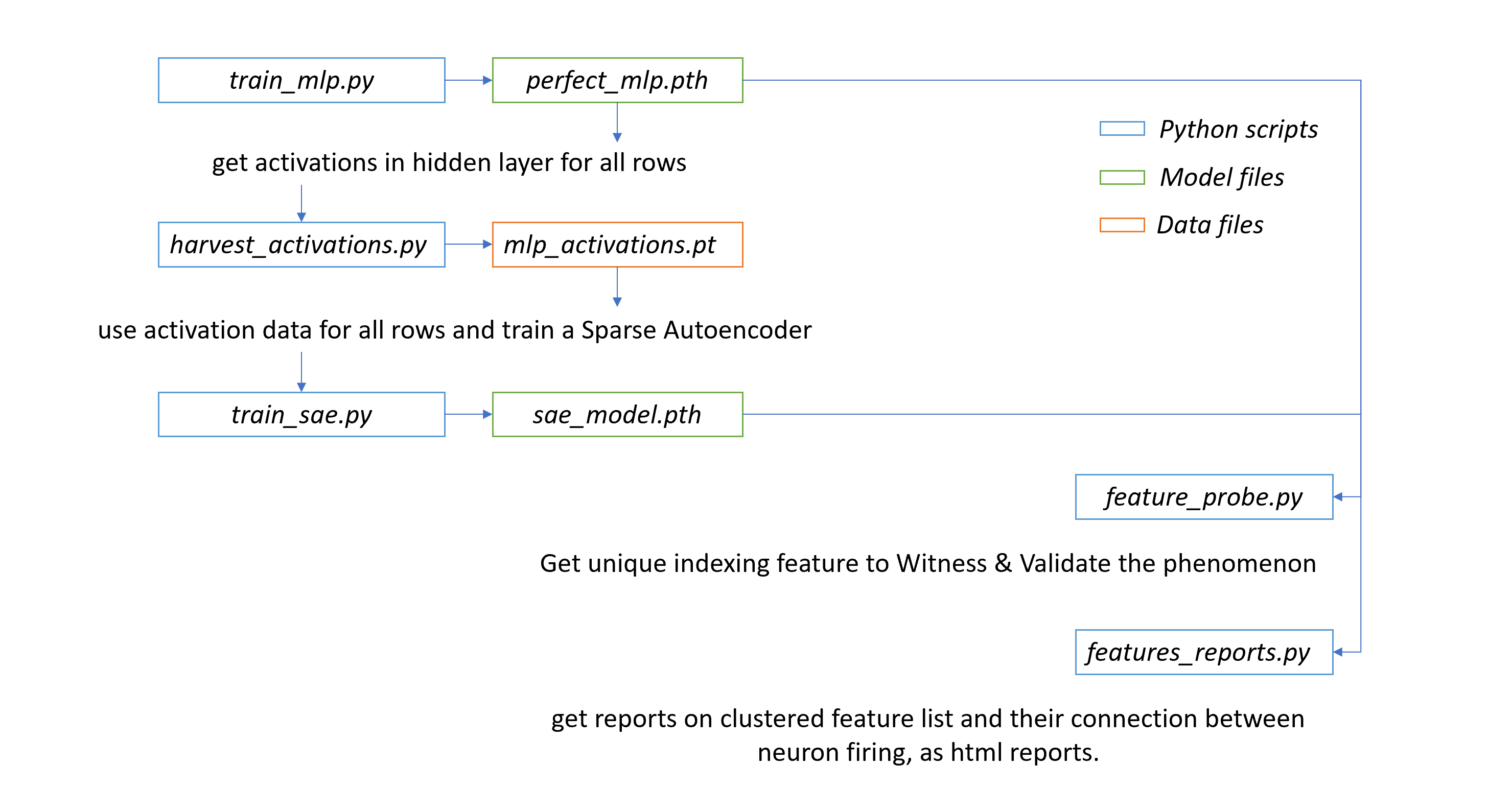
Dataset Generation: We use a math model to generate our data, that has 10x1 Inputs and 1x1 Output.
MLP Training: train_mlp.py optimizes the network to solve the math task, saving the "perfected" weights to perfect_mlp.pth.
Activation Harvesting: harvest_activations.py passes the training set through the frozen MLP. It "hooks" the 512-dim hidden layer and saves the result as mlp_activations.pt.
SAE Dictionary Learning: train_sae.py trains the Sparse Autoencoder on the harvested activations. The L1 penalty forces the SAE to use a sparse set of the 2048 available "dictionary" features to reconstruct the MLP's state.
Feature Probing: feature_probe.py evaluates specific inputs to identify which SAE features (e.g., #1883) correspond to specific mathematical indices.
Reporting: feature_reports.py aggregates all feature-to-neuron mappings into clustered HTML reports for global interpretability.
C:\Workspace\Git_Repos\monosemanticity-mlp-interpretability>workflow.bat
[1/7] Activating Environment...
[2/7] Generating Dataset...
Generating 8000 rows for mlp_train.xlsx...
Successfully saved mlp_train.xlsx
Generating 1000 rows for mlp_val.xlsx...
Successfully saved mlp_val.xlsx
Generating 1000 rows for mlp_test.xlsx...
Successfully saved mlp_test.xlsx
[3/7] Training MLP...
Epoch 50 | Val MSE: 0.709485
Epoch 100 | Val MSE: 0.813464
Epoch 150 | Val MSE: 0.447466
Epoch 200 | Val MSE: 0.347589
Epoch 250 | Val MSE: 0.199275
Epoch 300 | Val MSE: 0.185669
Epoch 350 | Val MSE: 0.190938
Epoch 400 | Val MSE: 0.154719
Epoch 450 | Val MSE: 0.150248
Epoch 500 | Val MSE: 0.147577
[4/7] Harvesting Activations...
Harvesting activations...
Success! Saved tensor of shape: torch.Size([8000, 512])
[5/7] Training Sparse Autoencoder (SAE)...
Loaded activations: torch.Size([8000, 512])
SAE Epoch [10/100] | Loss: 0.004299
SAE Epoch [20/100] | Loss: 0.003039
SAE Epoch [30/100] | Loss: 0.002528
SAE Epoch [40/100] | Loss: 0.002164
SAE Epoch [50/100] | Loss: 0.001973
SAE Epoch [60/100] | Loss: 0.001845
SAE Epoch [70/100] | Loss: 0.001711
SAE Epoch [80/100] | Loss: 0.001621
SAE Epoch [90/100] | Loss: 0.001613
SAE Epoch [100/100] | Loss: 0.001476
SAE training complete. Weights saved.
[6/7] Running Feature Probe...
--- Interpretability Report ---
Sample Input: [8, 9, 5, 1, 3, 2, 9, 4, 7, 1] | Expected Output: 8.0
MLP Output: 7.4849
Number of active SAE features: 62
Top Active Features (Monosemantic Candidates):
Feature #1649 | Activation: 0.6050
Feature #1440 | Activation: 0.5738
Feature #1608 | Activation: 0.4926
Feature #2028 | Activation: 0.3303
Feature # 725 | Activation: 0.3191
--- Interpretability Report ---
Sample Input: [8, 9, 5, 2, 3, 2, 8, 4, 7, 1] | Expected Output: 6.0
MLP Output: 5.6758
Number of active SAE features: 66
Top Active Features (Monosemantic Candidates):
Feature #1440 | Activation: 0.5455
Feature #1649 | Activation: 0.4891
Feature # 725 | Activation: 0.3875
Feature #1608 | Activation: 0.3647
Feature # 72 | Activation: 0.3016
--- Interpretability Report ---
Sample Input: [8, 9, 5, 3, 3, 2, 7, 4, 7, 1] | Expected Output: 4.0
MLP Output: 3.4448
Number of active SAE features: 60
Top Active Features (Monosemantic Candidates):
Feature #1440 | Activation: 0.5258
Feature # 725 | Activation: 0.4585
Feature #1649 | Activation: 0.4047
Feature #1478 | Activation: 0.2813
Feature # 72 | Activation: 0.2565
--- Interpretability Report ---
Sample Input: [8, 9, 5, 4, 3, 2, 5, 4, 7, 1] | Expected Output: 1.0
MLP Output: 0.8271
Number of active SAE features: 59
Top Active Features (Monosemantic Candidates):
Feature #1440 | Activation: 0.4882
Feature # 725 | Activation: 0.4855
Feature #1649 | Activation: 0.3640
Feature #1478 | Activation: 0.3147
Feature #1212 | Activation: 0.1984
--- Interpretability Report ---
Sample Input: [8, 9, 5, 5, 3, 2, 4, 4, 7, 1] | Expected Output: 1.0
MLP Output: 1.3972
Number of active SAE features: 64
Top Active Features (Monosemantic Candidates):
Feature # 725 | Activation: 0.4864
Feature #1440 | Activation: 0.4512
Feature #1649 | Activation: 0.3346
Feature #1478 | Activation: 0.3299
Feature #1212 | Activation: 0.3073
[7/7] Generating Feature Reports...
Tracing logic flow through the entire circuit...
Clean, centered report saved to circuit_trace_detailed.xlsx
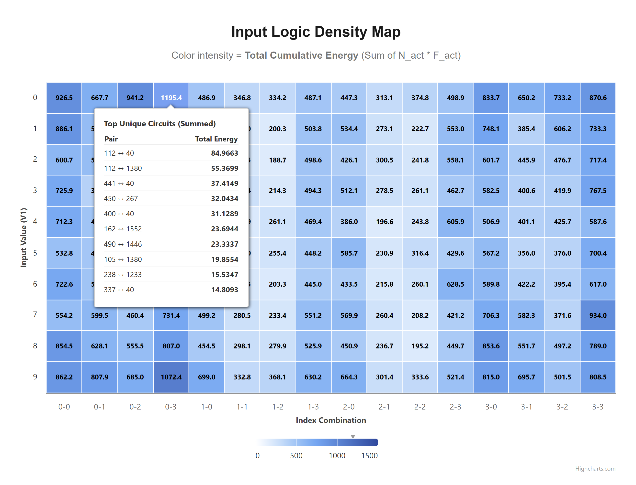
Logic heatmap saved to: C:\Workspace\Git_Repos\monosemanticity-mlp-interpretability\logic_circuit_map.html
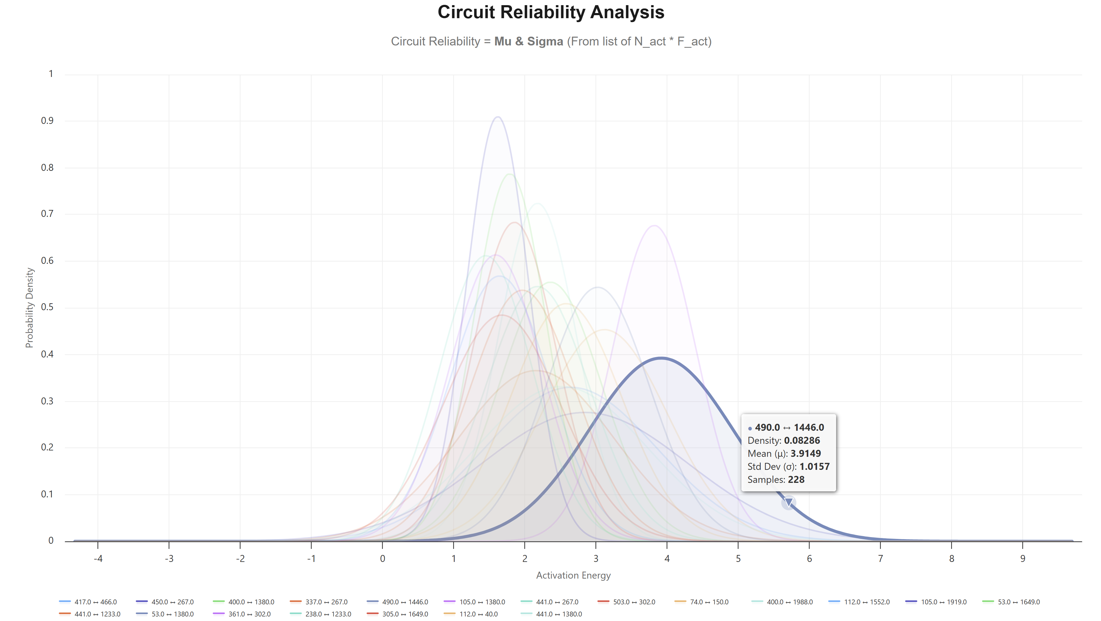
Interactive bell curve visualization saved
Total circuits: 1000
Sorted by: Mean (descending)
Default selection: First 10 circuits (highest means)
Stacked norm dist saved to: C:\Workspace\Git_Repos\monosemanticity-mlp-interpretability\circuit_bell_curves.html
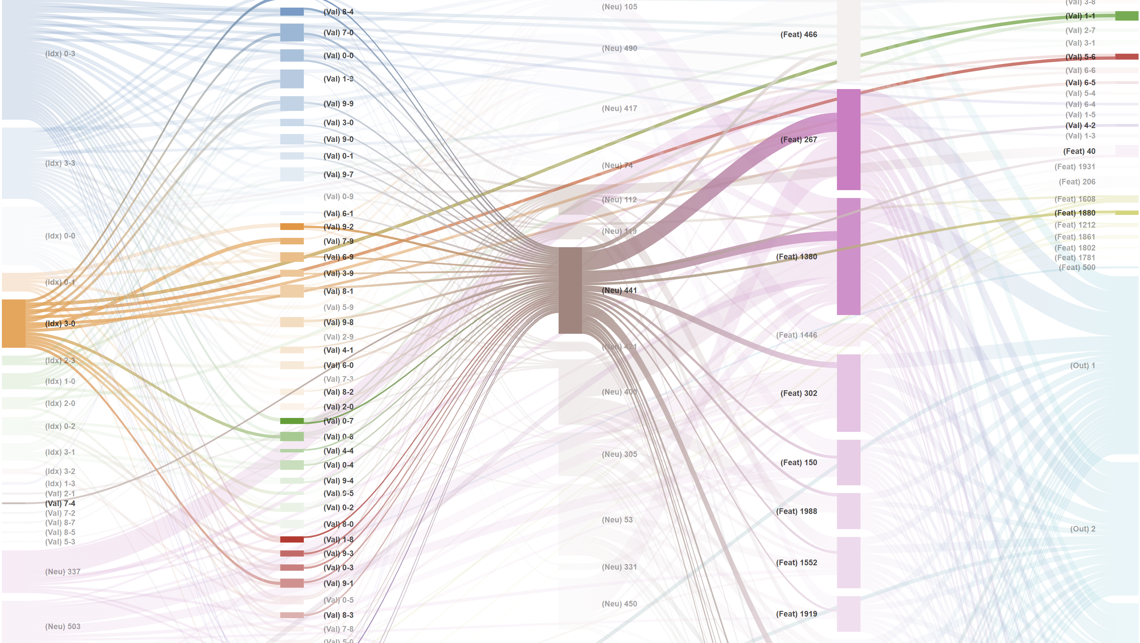
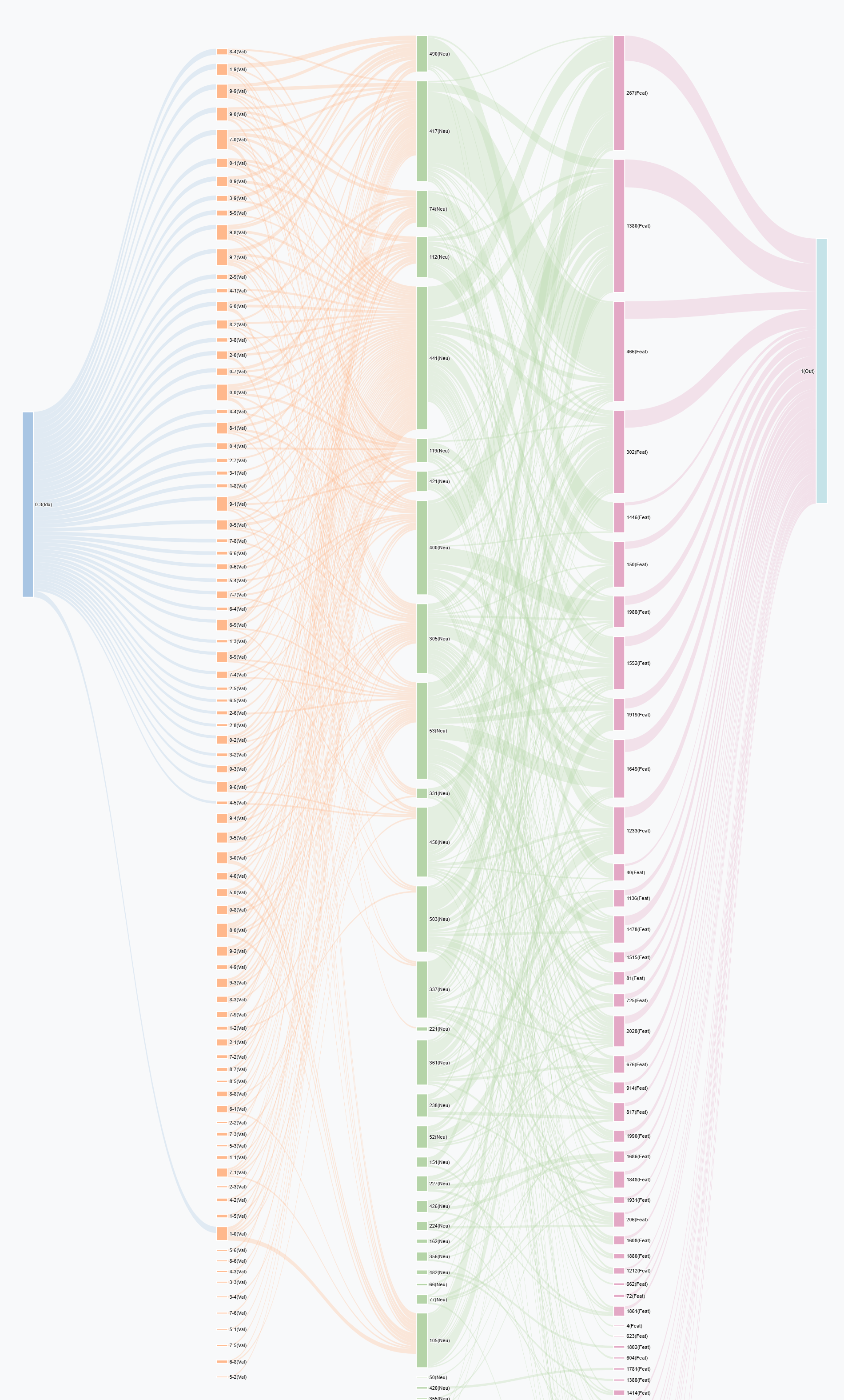
Sankey diagram saved to: C:\Workspace\Git_Repos\monosemanticity-mlp-interpretability\sankey_flow_diagram.html
Total nodes: 208
Total links: 1000
Plot height: 3150px
Layer distribution:
Layer 0 (Idx): 12 nodes
Layer 1 (Val): 90 nodes
Layer 2 (Neu): 34 nodes
Layer 3 (Feat): 62 nodes
Layer 4 (Out): 10 nodes
======================================================
Pipeline Complete: Monosemantic Features Identified.
======================================================
------------------------------------------------------
Execution Summary:
Started: 01:02:39
Finished: 01:23:48
Duration: 21 m 9 s
------------------------------------------------------
MLP Performance : The MLP demonstrated strong learning behavior, with the Validation MSE dropping significantly from 0.709 (Epoch 50) to a stable 0.147 (Epoch 500). The narrow delta between expected and actual outputs (e.g., 8.0 vs 7.48) confirms the model effectively captured the underlying mathematical logic of the dataset.
SAE Efficiency : The Sparse Autoencoder achieved an exceptionally low loss of 0.001476 by Epoch 100. This indicates the SAE has successfully learned to reconstruct the MLP’s 512-dimensional hidden activations using a sparse set of features without losing critical information.
The feature probing phase reveals a highly structured internal representation. We can infer the functional roles of specific features based on their activation patterns across samples:
Feature #1440 & #1649 (The "Core Logic" Features) : These features are consistently the top activations across all samples. They likely represent the primary arithmetic or logical operation required by the task.
Feature #725 (The "Inverse Correlation" Feature) : Notice that as the Expected Output decreases ($8.0 \to 1.0$), the activation of Feature #725 increases ($0.319 \to 0.486$). This suggests Feature #725 may be specialized in detecting or processing lower-magnitude results or specific input decrements.
Sparsity Constraints : With approximately 60-66 active features out of the latent space, the model is utilizing roughly 10-12% of its capacity per inference. This level of sparsity is ideal for identifying "monosemantic" units—features that do one specific job.
The pipeline successfully synthesized three distinct perspectives of the model's "brain":
The Logic Heatmap : Maps the raw input triggers to internal activation. (refer logic_circuit_map.html)
If you use this codebase for research, please cite the original paper that inspired this architecture:
Bricken, T., Templeton, A., Batson, J., Chen, B., Adler, J., Kotagi, A., ... & Olah, C. (2023). Towards Monosemanticity: Decomposing Language Models with Dictionary Learning. Transformer Circuits Thread.